Taking full advantage of a reduced workload these past few days, I found myself thinking of DMR again after stumbling across the Zumspot AMBE Server. That seemed like an excellent non-radio means of bringing up DMR, DSTAR or Fusion on any Windows box here at the house. So I placed an order and hopefully will be able to play around with it in a week or so.
Meanwhile, it seems like PA7LIM’s BlueDV is the software that many people are using with the AMBE Server or various USB Dongles, so I downloaded a copy in hopes of getting it to work with my old DV3K Dongle, something I had only used for DSTAR using DVTool. Since that used a AMBE3000R chip, I felt there was a small chance it might work with BlueDV, which would make it usable on DMR, Fusion, and DSTAR as well.
I was pleasantly surprised to find out it worked quite well, and within about 30 minutes of trying a few options, BlueDV was up and running.
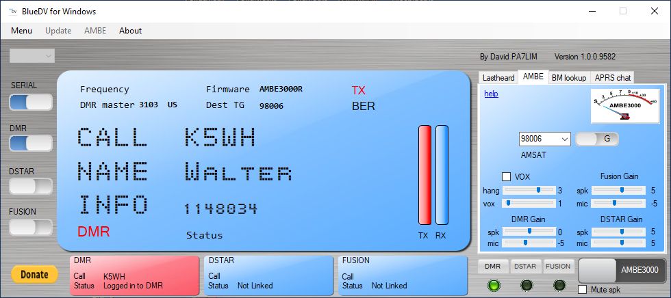
Chatting with Walter K5WH via the DMR 98006 AMSAT Talk Group
The setup was pretty simple. I guessed that the slower baud rate was used for the old device (located on COM6 on my PC), and assumed all the DMR ID settings would be mine (3144032). (Just a FYI, it appears the SETUP menu can’t be selected if any of the SERIAL, DMR, DSTAR, or FUSION switches are Active along the left side of the screen.)

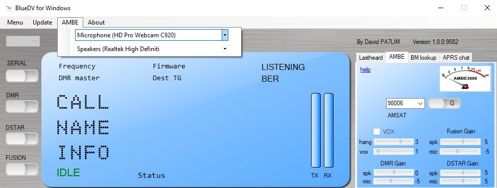
The only non-obvious thing to me was a need to setup the AMBE tab (along the top), as it was completely blank when I started things going. However, when I pulled down the choices I saw my mic and speaker selections which made perfect sense.
Finally I guessed that I needed to use the other AMBE tab to the right to select a talk group, and I set that to AMSAT 98006 (BrandMeister).
My last two stumbling blocks were forgetting that nothing would happen on DMR until I pressed “PTT” to get the Talk Group set. Now where is that PTT button???? That took a tad bit of exploring and I found a YouTube video from TechMinds that revealed the magic solution — use the bottom right “AMBE3000” slider by clicking on it to turn TX on, and clicking again to turn TX off!
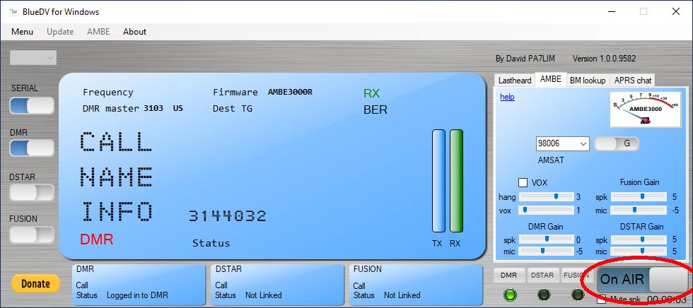
The “PTT” in AMBE3000 mode is the slider in the lower right corner. Click for PTT
I look forward to trying this with the AMBE Server — that will make this a solution I can run from pretty much everywhere.